Lists

4. Lists#

Python provides a powerful set of tools to create and manipulate lists of data. In this part, we take a deep dive into the Python list type. This includes mutability, list methods, and slicing.

Then we use Python lists to implement and optimize the Sieve of Eratosthenes, which will produce a list of all prime numbers up to a big number (like 10 million) in a snap. Along the way, we introduce some Python techniques for data analysis and visualization.

4.1. Primality testing#

Before diving into lists, we recall the brute force primality test that we created in the last lesson. To test whether a number n is prime, we can simply check for factors. This yields the following primality test.

def is_prime(n):
    '''
    Checks whether the argument n is a prime number.
    Uses a brute force search for factors between 1 and n.
    '''
    for j in range(2,n):  # the range of numbers 2,3,...,n-1.
        if n%j == 0:  # is n divisible by j?
            print("{} is a factor of {}.".format(j,n))
            return False
    return True

We can also implement this test with a while loop instead of a for loop. This doesn’t make much of a difference, in Python 3.x. (In Python 2.x, this would save memory).

def is_prime(n):
    '''
    Checks whether the argument n is a prime number.
    Uses a brute force search for factors between 1 and n.
    '''
    j = 2
    while j < n:  # j will proceed through the list of numbers 2,3,...,n-1.
        if n%j == 0:  # is n divisible by j?
            print("{} is a factor of {}.".format(j,n))
            return False
        j = j + 1  # There's a Python abbreviation for this:  j += 1.
    return True

is_prime(10001)

73 is a factor of 10001.

False

is_prime(101)

True

If $n$ is a prime number, then the is_prime(n) function will iterate through all the numbers between $2$ and $n-1$. But this is overkill! Indeed, if $n$ is not prime, it will have a factor between $2$ and the square root of $n$. This is because factors come in pairs: if $ab = n$, then one of the factors, $a$ or $b$, must be less than or equal to the square root of $n$. So it suffices to search for factors up to (and including) the square root of $n$.

Even though we’ve made our own sqrt function, we load a fast one from the standard math package. You can use this for square roots, trig functions, logs, and more. Click the previous link for documentation. This package doesn’t load automatically when you start Python, so you have to load it with a little Python code.

from math import sqrt

This command imports the square root function (sqrt) from the package called math. Now you can find square roots.

sqrt(1000)

31.622776601683793

There are a few different ways to import functions from packages. The above syntax is a good starting point, but sometimes problems can arise if different packages have functions with the same name. Here are a few methods of importing the sqrt function and how they differ.

from math import sqrt: After this command, sqrt will refer to the function from the math package (overriding any previous definition).

import math: After this command, all the functions from the math package will be imported. But to call sqrt, you would type a command like math.sqrt(1000). This is convenient if there are potential conflicts with other packages.

from math import *: After this command, all the functions from the math package will be imported. To call them, you can access them directly with a command like sqrt(1000). This can easily cause conflicts with other packages, since packages can have hundreds of functions in them!

import math as mth: Some people like abbreviations. This imports all the functions from the math package. To call one, you type a command like mth.sqrt(1000).

import math
math.sqrt(1000)

31.622776601683793

factorial(10)  # This will cause an error!

---------------------------------------------------------------------------
NameError                                 Traceback (most recent call last)
Cell In[8], line 1
----> 1 factorial(10)  # This will cause an error!

NameError: name 'factorial' is not defined

math.factorial(10)  # This is ok, since the math package comes with a function called factorial.

Now let’s improve our is_prime(n) function by searching for factors only up to the square root of the number n. We consider two options.

def is_prime_slow(n):
    '''
    Checks whether the argument n is a prime number.
    Uses a brute force search for factors between 2 and sqrt(n).
    '''
    j = 2
    while j <= sqrt(n):  # j will proceed through the list of numbers 2,3,... up to sqrt(n).
        if n%j == 0:  # is n divisible by j?
            print("{} is a factor of {}.".format(j,n))
            return False
        j = j + 1  # There's a Python abbreviation for this:  j += 1.
    return True

def is_prime_fast(n):
    '''
    Checks whether the argument n is a prime number.
    Uses a brute force search for factors between 2 and sqrt(n).
    '''
    j = 2
    root_n = sqrt(n)
    while j <= root_n:  # j will proceed through the list of numbers 2,3,... up to sqrt(n).
        if n%j == 0:  # is n divisible by j?
            print("{} is a factor of {}.".format(j,n))
            return False
        j = j + 1  # There's a Python abbreviation for this:  j += 1.
    return True

is_prime_fast(1000003)

True

is_prime_slow(1000003)

True

I’ve chosen function names with “fast” and “slow” in them. But what makes them faster or slower? Are they faster than the original? And how can we tell?

Python comes with a great set of tools for these questions. The simplest (for the user) are the time utilities. By placing the magic %timeit before a command, Python does something like the following:

Python makes a little container in your computer devoted to the computations, to avoid interference from other running programs if possible.
Python executes the command lots and lots of times.
Python averages the amount of time taken for each execution.

Give it a try below, to compare the speed of the functions is_prime (the original) with the new is_prime_fast and is_prime_slow. Note that the %timeit commands might take a little while.

Warning! Before running the is_prime_fast and is_prime_slow functions within %timeit, please remove all print statements from the functions and recompile them. Otherwise, you might end up printing a million things in your browser window, possibly crashing your computer.

%timeit is_prime_fast(1000003)

37.3 µs ± 181 ns per loop (mean ± std. dev. of 7 runs, 10,000 loops each)

%timeit is_prime_slow(1000003)

58.2 µs ± 1.77 µs per loop (mean ± std. dev. of 7 runs, 10,000 loops each)

%timeit is_prime(1000003)

29.3 ms ± 376 µs per loop (mean ± std. dev. of 7 runs, 10 loops each)

Time is measured in seconds, milliseconds (1 ms = 1/1000 second), microseconds (1 µs = 1/1,000,000 second), and nanoseconds (1 ns = 1/1,000,000,000 second). So it might appear at first that is_prime is the fastest, or about the same speed. But check the units! The other two approaches are about a thousand times faster! How much faster were they on your computer?

is_prime_fast(10000000000037)  # Don't try this with `is_prime` unless you want to wait for a long time!

True

Indeed, the is_prime_fast(n) function will go through a loop of length about sqrt(n) when n is prime. But is_prime(n) will go through a loop of length about n. Since sqrt(n) is much less than n, especially when n is large, the is_prime_fast(n) function is much faster.

Between is_prime_fast and is_prime_slow, the difference is that the fast version precomputes the square root sqrt(n) before going through the loop, where the slow version repeats the sqrt(n) every time the loop is repeated. Indeed, writing while j <= sqrt(n): suggests that Python might execute sqrt(n) every time to check. This might lead to Python computing the same square root a million times… unnecessarily!

A basic principle of programming is to avoid repetition. If you have the memory space, just compute once and store the result. It will probably be faster to pull the result out of memory than to compute it again.

Python does tend to be pretty smart, however. It’s possible that Python is precomputing sqrt(n) even in the slow loop, just because it’s clever enough to tell in advance that the same thing is being computed over and over again. This depends on your Python version and takes place behind the scenes. If you want to figure it out, there’s a whole set of tools (for advanced programmers) like the disassembler to figure out what Python is doing.

If you feel like looking under the hood, the next few lines will display the is_prime_fast and is_prime_slow functions to bytecode. Can you see how the sqrt(n) computation is carried out differently?

from dis import dis

dis(is_prime_fast)

  1           0 RESUME                   0

  6           2 LOAD_CONST               1 (2)
              4 STORE_FAST               1 (j)

  7           6 LOAD_GLOBAL              1 (NULL + sqrt)
             18 LOAD_FAST                0 (n)
             20 PRECALL                  1
             24 CALL                     1
             34 STORE_FAST               2 (root_n)

  8          36 LOAD_FAST                1 (j)
             38 LOAD_FAST                2 (root_n)
             40 COMPARE_OP               1 (<=)
             46 POP_JUMP_FORWARD_IF_FALSE    57 (to 162)

  9     >>   48 LOAD_FAST                0 (n)
             50 LOAD_FAST                1 (j)
             52 BINARY_OP                6 (%)
             56 LOAD_CONST               2 (0)
             58 COMPARE_OP               2 (==)
             64 POP_JUMP_FORWARD_IF_FALSE    37 (to 140)

 10          66 LOAD_GLOBAL              3 (NULL + print)
             78 LOAD_CONST               3 ('{} is a factor of {}.')
             80 LOAD_METHOD              2 (format)
            102 LOAD_FAST                1 (j)
            104 LOAD_FAST                0 (n)
            106 PRECALL                  2
            110 CALL                     2
            120 PRECALL                  1
            124 CALL                     1
            134 POP_TOP

 11         136 LOAD_CONST               4 (False)
            138 RETURN_VALUE

 12     >>  140 LOAD_FAST                1 (j)
            142 LOAD_CONST               5 (1)
            144 BINARY_OP                0 (+)
            148 STORE_FAST               1 (j)

  8         150 LOAD_FAST                1 (j)
            152 LOAD_FAST                2 (root_n)
            154 COMPARE_OP               1 (<=)
            160 POP_JUMP_BACKWARD_IF_TRUE    57 (to 48)

 13     >>  162 LOAD_CONST               6 (True)
            164 RETURN_VALUE

dis(is_prime_slow)

  1           0 RESUME                   0

  6           2 LOAD_CONST               1 (2)
              4 STORE_FAST               1 (j)

  7           6 LOAD_FAST                1 (j)
              8 LOAD_GLOBAL              1 (NULL + sqrt)
             20 LOAD_FAST                0 (n)
             22 PRECALL                  1
             26 CALL                     1
             36 COMPARE_OP               1 (<=)
             42 POP_JUMP_FORWARD_IF_FALSE    70 (to 184)

  8     >>   44 LOAD_FAST                0 (n)
             46 LOAD_FAST                1 (j)
             48 BINARY_OP                6 (%)
             52 LOAD_CONST               2 (0)
             54 COMPARE_OP               2 (==)
             60 POP_JUMP_FORWARD_IF_FALSE    37 (to 136)

  9          62 LOAD_GLOBAL              3 (NULL + print)
             74 LOAD_CONST               3 ('{} is a factor of {}.')
             76 LOAD_METHOD              2 (format)
             98 LOAD_FAST                1 (j)
            100 LOAD_FAST                0 (n)
            102 PRECALL                  2
            106 CALL                     2
            116 PRECALL                  1
            120 CALL                     1
            130 POP_TOP

 10         132 LOAD_CONST               4 (False)
            134 RETURN_VALUE

 11     >>  136 LOAD_FAST                1 (j)
            138 LOAD_CONST               5 (1)
            140 BINARY_OP                0 (+)
            144 STORE_FAST               1 (j)

  7         146 LOAD_FAST                1 (j)
            148 LOAD_GLOBAL              1 (NULL + sqrt)
            160 LOAD_FAST                0 (n)
            162 PRECALL                  1
            166 CALL                     1
            176 COMPARE_OP               1 (<=)
            182 POP_JUMP_BACKWARD_IF_TRUE    70 (to 44)

 12     >>  184 LOAD_CONST               6 (True)
            186 RETURN_VALUE

is_prime_fast(10**14 + 37) # This might get a bit of delay.

1858741 is a factor of 100000000000037.

False

Now we have a function is_prime_fast(n) that is speedy for numbers n in the trillions! You’ll probably start to hit a delay around $10^{15}$ or so, and the delays will become intolerable if you add too many more digits. In a future lesson, we will see a different primality test that will be essentially instant even for numbers around $10^{1000}$!

4.2. List manipulation#

We have already (briefly) encountered the list type in Python. Recall that the range command produces a range, which can be used to produce a list. For example, list(range(10)) produces the list [0,1,2,3,4,5,6,7,8,9]. You can also create your own list by a writing out its terms, e.g. L = [4,7,10].

Here we work with lists, and a very Pythonic approach to list manipulation. With practice, this can be a powerful tool to write fast algorithms, exploiting the hard-wired capability of your computer to shift and slice large chunks of data. Our eventual application will be to implement the Sieve of Eratosthenes, producing a long list of prime numbers (without using any is_prime test along the way).

We begin by creating a list to play with. We mix numbers and strings… just for fun.

L = [0,'one',2,'three',4,'five',6,'seven',8,'nine',10]

4.2.1. List terms and indices#

Notice that the entries in a list can be of any type. The above list L has some integer entries and some string entries. Lists are ordered in Python, starting at zero. One can access the $n^{th}$ entry in a list with a command like L[n].

L[3]

'three'

print(L[3])  # Note that Python has slightly different approaches to the print-function, and the output above.

three

print(L[4])  # We will use the print function, because it makes our printing intentions clear.

print(L[0])

The location of an entry is called its index. So at the index 3, the list L stores the entry three. Note that the same entry can occur in many places in a list. E.g. [7,7,7] is a list with 7 at the zeroth, first, and second index.

# L = [0,'one',2,'three',4,'five',6,'seven',8,'nine',10]
print(L[-1])
print(L[-2])

10
nine

The last bit of code demonstrates a cool Python trick. The “-1st” entry in a list refers to the last entry. The “-2nd entry” refers to the second-to-last entry, and so on. It gives a convenient way to access both sides of the list, even if you don’t know how long it is.

Of course, you can use Python to find out how long a list is.

len(L)

You can also use Python to find the sum of a list of numbers.

sum([1,2,3,4,5])

sum(range(5))  # Be careful.  This is the sum of which numbers?  # The sum function can take lists or ranges.

4.2.2. List slicing#

Slicing lists allows us to create new lists (or ranges) from old lists (or ranges), by chopping off one end or the other, or even slicing out entries at a fixed interval. The simplest syntax has the form L[a:b] where a denotes the index of the starting entry and index of the final entry is one less than b. It is best to try a few examples to get a feel for it.

Slicing a list with a command like L[a:b] doesn’t actually change the original list L. It just extracts some terms from the list and outputs those terms. Soon enough, we will change the list L using a list assignment.

# L = [0,'one',2,'three',4,'five',6,'seven',8,'nine',10]
L[0:5]

[0, 'one', 2, 'three', 4]

L[5:11]  # Notice that L[0:5] and L[5:11] together recover the whole list.

['five', 6, 'seven', 8, 'nine', 10]

L[3:7]

['three', 4, 'five', 6]

This continues the strange (for beginners) Python convention of starting at the first number and ending just before the last number. Compare to range(3,7), for example.

The command L[0:5] can be replaced by L[:5] to abbreviate. The empty opening index tells Python to start at the beginning. Similarly, the command L[5:11] can be replaced by L[5:]. The empty closing index tells Python to end the slice and the end. This is helpful if one doesn’t know where the list ends.

L[:5]

[0, 'one', 2, 'three', 4]

L[3:]

['three', 4, 'five', 6, 'seven', 8, 'nine', 10]

Just like the range command, list slicing can take an optional third argument to give a step size. To understand this, see the command below.

L[2:10]

[2, 'three', 4, 'five', 6, 'seven', 8, 'nine']

L[2:10:3]

[2, 'five', 8]

If, in this three-argument syntax, the first or second argument is absent, then the slice starts at the beginning of the list or ends at the end of the list accordingly.

L  # Just a reminder.  We haven't modified the original list!

[0, 'one', 2, 'three', 4, 'five', 6, 'seven', 8, 'nine', 10]

L[:9:3]  # Start at zero, go up to (but not including) 9, by steps of 3.

[0, 'three', 6]

L[2: :3] # Start at two, go up through the end of the list, by steps of 3.

[2, 'five', 8]

L[::3]  # Start at zero, go up through the end of the list, by steps of 3.

[0, 'three', 6, 'nine']

4.2.3. Changing list slices#

Not only can we extract and study terms or slices of a list, we can change them by assignment. The simplest case would be changing a single term of a list.

print(L) # Start with the list L.

[0, 'one', 2, 'three', 4, 'five', 6, 'seven', 8, 'nine', 10]

L[5] = 'Bacon!'

print(L)  # What do you think L is now?

[0, 'one', 2, 'three', 4, 'Bacon!', 6, 'seven', 8, 'nine', 10]

print(L[2::3]) # What do you think this will do?

[2, 'Bacon!', 8]

We can change an entire slice of a list with a single assignment. Let’s change the first two terms of L in one line.

L[:2] = ['Pancakes', 'Ham']  # What was L[:2] before?

print(L) # Oh... what have we done!

['Pancakes', 'Ham', 2, 'three', 4, 'Bacon!', 6, 'seven', 8, 'nine', 10]

L[0]

'Pancakes'

We can change a slice of a list with a single assignment, even when that slice does not consist of consecutive terms. Try to predict what the following commands will do.

print(L)  # Let's see what the list looks like before.

['Pancakes', 'Ham', 2, 'three', 4, 'Bacon!', 6, 'seven', 8, 'nine', 10]

L[::2] = ['A','B','C','D','E','F']  # What was L[::2] before this assignment? 

print(L)  # What do you predict?

['A', 'Ham', 'B', 'three', 'C', 'Bacon!', 'D', 'seven', 'E', 'nine', 'F']

4.3. List methods#

A method is a function that is attached to an object. We have already used one method: the format method that is attached to all strings. You might have seen the replace method for strings too. Note that single-quotes 'Hello' or double-quotes "Hello" can be used for strings.

"Hello {}!".format('programming student')

'Hello programming student!'

"Programming is fun!".replace('fun','lit')

'Programming is lit!'

List methods are functions attached to lists. Some useful methods include append and sort. A fuller listing can be found at the official documentation.

L = [1,2,3]
L.append(4)
print(L)

[1, 2, 3, 4]

The append method can be used to add new items to the end of a list. But be careful if you want to add multiple items!

L.append([5,6])
print(L)

[1, 2, 3, 4, [5, 6]]

We can use L.remove(x) to remove the first item from the list L whose value is equal to x. It raises a ValueError if there is no such item.

L.remove([5,6]) 
print(L)

[1, 2, 3, 4]

L.extend([5,6]) # extend the list by appending all the items from the list [5,6]
print(L)

[1, 2, 3, 4, 5, 6]

Behind the scenes, methods are functions which have a special input parameter called self. So when you use a command like L.append(4), you are effectively running append(L, 4). The self parameter is the object the method is attached to.

Like all functions, methods have outputs too. But what can be confusing is that methods can modify self and can sometimes return None.

print([1,2,3].append(4))
print("123".replace("3","4"))

None
124

This is very confusing at first! The list append method does change self by appending something to self. But as a function, it returns None.

On the other hand, the string replace method does not change self and instead returns the modified string.

This will make more sense after we study mutable and immutable types. Lists are mutable (and thus are often changed by their methods). Strings are immutable, and so changes are effected by producing new strings. Another example of a string method is sort(). The only parameter of sort is self, and so nothing needs to go between the parentheses.

L = [4,2,1]  # Make a list.
L.sort()  # Sort the list.  This *changes* L and returns None.
print(L)  # Let's see what L is now.

[1, 2, 4]

L = ['Ukelele', 'Apple', 'Dog', 'Cat' ]
L.sort()
print(L)

['Apple', 'Cat', 'Dog', 'Ukelele']

Sorting numbers is possible, because the Python operator < is defined for numbers. Sorting strings is possible, because the Python operator < is interpreted alphabetically among strings. If you mix types, Python might not know how to behave… you’ll get a TypeError.

L = [1,'Apple', 3.14]
L.sort()
print(L)

---------------------------------------------------------------------------
TypeError                                 Traceback (most recent call last)
/Users/ssuzana/python-programming-for-math/content/03-lists.ipynb Cell 99 line 2
      <a href='vscode-notebook-cell:/Users/ssuzana/python-programming-for-math/content/03-lists.ipynb#Y201sZmlsZQ%3D%3D?line=0'>1</a> L = [1,'Apple', 3.14]
----> <a href='vscode-notebook-cell:/Users/ssuzana/python-programming-for-math/content/03-lists.ipynb#Y201sZmlsZQ%3D%3D?line=1'>2</a> L.sort()
      <a href='vscode-notebook-cell:/Users/ssuzana/python-programming-for-math/content/03-lists.ipynb#Y201sZmlsZQ%3D%3D?line=2'>3</a> print(L)

TypeError: '<' not supported between instances of 'str' and 'int'

4.4. Sieve of Eratosthenes#

The Sieve of Eratosthenes (hereafter called “the sieve”) is a very fast way of producing long lists of primes, without doing repeated primality checking. The basic idea is to start with all of the natural numbers, and successively filter out, or sieve, the multiples of 2, then the multiples of 3, then the multiples of 5, etc., until only primes are left. You can read more about the sieve, and experimental number theory, at The Conversation.

Using list slicing, we can carry out this sieving process efficiently. And with a few more tricks we encounter here, we can carry out the Sieve very efficiently.

The first approach we introduce is a bit naive, but is a good starting place. We will begin with a list of numbers up to 100, and sieve out the appropriate multiples of 2,3,5,7.

primes = list(range(100)) # Let's start with the numbers 0...99.

Now, to “filter”, i.e., to say that a number is not prime, let’s just change the number to the value None.

primes[0] = None # Zero is not prime.
primes[1] = None # One is not prime.
print(primes) # What have we done?

[None, None, 2, 3, 4, 5, 6, 7, 8, 9, 10, 11, 12, 13, 14, 15, 16, 17, 18, 19, 20, 21, 22, 23, 24, 25, 26, 27, 28, 29, 30, 31, 32, 33, 34, 35, 36, 37, 38, 39, 40, 41, 42, 43, 44, 45, 46, 47, 48, 49, 50, 51, 52, 53, 54, 55, 56, 57, 58, 59, 60, 61, 62, 63, 64, 65, 66, 67, 68, 69, 70, 71, 72, 73, 74, 75, 76, 77, 78, 79, 80, 81, 82, 83, 84, 85, 86, 87, 88, 89, 90, 91, 92, 93, 94, 95, 96, 97, 98, 99]

Now let’s filter out the multiples of 2, starting at 4. This is the slice primes[4::2]

primes[4::2] = [None] * len(primes[4::2])  # The right side is a list of Nones, of the necessary length.
print(primes) # What have we done?

[None, None, 2, 3, None, 5, None, 7, None, 9, None, 11, None, 13, None, 15, None, 17, None, 19, None, 21, None, 23, None, 25, None, 27, None, 29, None, 31, None, 33, None, 35, None, 37, None, 39, None, 41, None, 43, None, 45, None, 47, None, 49, None, 51, None, 53, None, 55, None, 57, None, 59, None, 61, None, 63, None, 65, None, 67, None, 69, None, 71, None, 73, None, 75, None, 77, None, 79, None, 81, None, 83, None, 85, None, 87, None, 89, None, 91, None, 93, None, 95, None, 97, None, 99]

Now we filter out the multiples of 3, starting at 9.

primes[9::3] = [None] * len(primes[9::3])  # The right side is a list of Nones, of the necessary length.
print(primes) # What have we done?

[None, None, 2, 3, None, 5, None, 7, None, None, None, 11, None, 13, None, None, None, 17, None, 19, None, None, None, 23, None, 25, None, None, None, 29, None, 31, None, None, None, 35, None, 37, None, None, None, 41, None, 43, None, None, None, 47, None, 49, None, None, None, 53, None, 55, None, None, None, 59, None, 61, None, None, None, 65, None, 67, None, None, None, 71, None, 73, None, None, None, 77, None, 79, None, None, None, 83, None, 85, None, None, None, 89, None, 91, None, None, None, 95, None, 97, None, None]

Next the multiples of 5, starting at 25 (the first multiple of 5 greater than 5 that’s left!)

primes[25::5] = [None] * len(primes[25::5])  # The right side is a list of Nones, of the necessary length.
print(primes) # What have we done?

[None, None, 2, 3, None, 5, None, 7, None, None, None, 11, None, 13, None, None, None, 17, None, 19, None, None, None, 23, None, None, None, None, None, 29, None, 31, None, None, None, None, None, 37, None, None, None, 41, None, 43, None, None, None, 47, None, 49, None, None, None, 53, None, None, None, None, None, 59, None, 61, None, None, None, None, None, 67, None, None, None, 71, None, 73, None, None, None, 77, None, 79, None, None, None, 83, None, None, None, None, None, 89, None, 91, None, None, None, None, None, 97, None, None]

Finally, the multiples of 7, starting at 49 (the first multiple of 7 greater than 7 that’s left!)

primes[49::7] = [None] * len(primes[49::7])  # The right side is a list of Nones, of the necessary length.
print(primes) # What have we done?

[None, None, 2, 3, None, 5, None, 7, None, None, None, 11, None, 13, None, None, None, 17, None, 19, None, None, None, 23, None, None, None, None, None, 29, None, 31, None, None, None, None, None, 37, None, None, None, 41, None, 43, None, None, None, 47, None, None, None, None, None, 53, None, None, None, None, None, 59, None, 61, None, None, None, None, None, 67, None, None, None, 71, None, 73, None, None, None, None, None, 79, None, None, None, 83, None, None, None, None, None, 89, None, None, None, None, None, None, None, 97, None, None]

What’s left? A lot of Nones and the prime numbers up to 100. We have successfully sieved out all the nonprime numbers in the list, using just four sieving steps (and setting 0 and 1 to None manually).

But there’s a lot of room for improvement, from beginning to end!

The format of the end result is not so nice.
We had to sieve each step manually. It would be much better to have a function prime_list(n) which would output a list of primes up to n without so much supervision.
The memory usage will be large, if we need to store all the numbers up to a large n at the beginning.

We solve these problems in the following way.

We will use a list of booleans rather than a list of numbers. The ending list will have a True value at prime indices and a False value at composite indices. This reduces the memory usage and increases the speed.
A where function (explained soon) will make the desired list of primes after everything else is done.
We will proceed through the sieving steps algorithmically rather than entering each step manually.

Here is a somewhat efficient implementation of the Sieve in Python.

from math import sqrt
def isprime_list(n):
    ''' 
    Return a list of length n+1
    with Trues at prime indices and Falses at composite indices.
    '''
    flags = [True] * (n+1)  # A list [True, True, True,...] to start.
    flags[0] = False  # Zero is not prime.  So its flag is set to False.
    flags[1] = False  # One is not prime.  So its flag is set to False.
    p = 2  # The first prime is 2.  And we start sieving by multiples of 2.
    
    while p <= sqrt(n):  # We only need to sieve by p is p <= sqrt(n).
        if flags[p]:  # We sieve the multiples of p if flags[p]=True.
            flags[p*p::p] = [False] * len(flags[p*p::p]) # Sieves out multiples of p, starting at p*p.
        p = p + 1 # Try the next value of p.
        
    return flags

print(isprime_list(100))

[False, False, True, True, False, True, False, True, False, False, False, True, False, True, False, False, False, True, False, True, False, False, False, True, False, False, False, False, False, True, False, True, False, False, False, False, False, True, False, False, False, True, False, True, False, False, False, True, False, False, False, False, False, True, False, False, False, False, False, True, False, True, False, False, False, False, False, True, False, False, False, True, False, True, False, False, False, False, False, True, False, False, False, True, False, False, False, False, False, True, False, False, False, False, False, False, False, True, False, False, False]

If you look carefully at the list of booleans, you will notice a True value at the 2nd index, the 3rd index, the 5th index, the 7th index, etc.. The indices where the values are True are precisely the prime indices. Since booleans take the smallest amount of memory of any data type (one bit of memory per boolean), your computer can carry out the isprime_list(n) function even when n is very large.

To be more precise, there are 8 bits in a byte. There are 1024 bytes (about 1000) in a kilobyte. There are 1024 kilobytes in a megabyte. There are 1024 megabytes in a gigabyte. Therefore, a gigabyte of memory is enough to store about 8 billion bits. That’s enough to store the result of isprime_list(n) when n is about 8 billion. Not bad! And your computer probably has 4 or 8 or 12 or 16 gigabytes of memory to use.

To transform the list of booleans into a list of prime numbers, we create a function called where. This function uses another Python technique called list comprehension. We discuss this technique later in this lesson, so just use the where function as a tool for now, or read about list comprehension if you’re curious.

def where(L):
    '''
    Take a list of booleans as input and
    outputs the list of indices where True occurs.
    '''
    return [n for n in range(len(L)) if L[n]]
    

Combined with the isprime_list function, we can produce long lists of primes.

print(where(isprime_list(100)))

[2, 3, 5, 7, 11, 13, 17, 19, 23, 29, 31, 37, 41, 43, 47, 53, 59, 61, 67, 71, 73, 79, 83, 89, 97]

Let’s push it a bit further. How many primes are there between 1 and 1 million? We can figure this out in three steps:

Create the isprime_list.
Use where to get the list of primes.
Find the length of the list of primes.

But it’s better to do it in two steps.

Create the isprime_list.
Sum the list! (Note that True is 1, for the purpose of summation!)

sum(isprime_list(1000000))  # The number of primes up to a million!

%timeit isprime_list(10**6)  # 1000 ms = 1 second.

24.2 ms ± 290 µs per loop (mean ± std. dev. of 7 runs, 10 loops each)

%timeit sum(isprime_list(10**6))

27.5 ms ± 175 µs per loop (mean ± std. dev. of 7 runs, 10 loops each)

This isn’t too bad! It takes a fraction of a second to identify the primes up to a million, and a smaller fraction of a second to count them! But we can do a little better.

The first improvement is to take care of the even numbers first. If we count carefully, then the sequence 4,6,8,…,n (ending at n-1 if n is odd) has the floor of (n-2)/2 terms. Thus the line flags[4::2] = [False] * ((n-2)//2) will set all the flags to False in the sequence 4,6,8,10,… From there, we can begin sieving by odd primes starting with 3.

The next improvement is that, since we’ve already sieved out all the even numbers (except 2), we don’t have to sieve out again by even multiples. So when sieving by multiples of 3, we don’t have to sieve out 9,12,15,18,21,etc.. We can just sieve out 9,15,21,etc.. When p is an odd prime, this can be taken care of with the code flags[p*p::2*p] = [False] * len(flags[p*p::2*p]).

def isprime_list(n):
    ''' 
    Return a list of length n+1
    with Trues at prime indices and Falses at composite indices.
    '''
    flags = [True] * (n+1)  # A list [True, True, True,...] to start.
    flags[0] = False  # Zero is not prime.  So its flag is set to False.
    flags[1] = False  # One is not prime.  So its flag is set to False.
    flags[4::2] = [False] * ((n-2)//2)
    p = 3
    while p <= sqrt(n):  # We only need to sieve by p is p <= sqrt(n).
        if flags[p]:  # We sieve the multiples of p if flags[p]=True.
            flags[p*p::2*p] = [False] * len(flags[p*p::2*p]) # Sieves out multiples of p, starting at p*p.
        p = p + 2 # Try the next value of p.  Note that we can proceed only through odd p!
        
    return flags

%timeit sum(isprime_list(10**6))  # How much did this speed it up?

17.3 ms ± 97.3 µs per loop (mean ± std. dev. of 7 runs, 100 loops each)

Another modest improvement is the following. In the code above, the program counts the terms in sequences like 9,15,21,27,…, in order to set them to False. This is accomplished with the length command len(flags[p*p::2*p]). But that length computation is a bit too intensive. A bit of algebraic work shows that the length is given formulaically in terms of p and n by the formula:

\[len = \left\lfloor \frac{n - p^2 - 1}{2p} \right\rfloor + 1\]

(Here $\lfloor x \rfloor$ denotes the floor function, i.e., the result of rounding down.) Putting this into the code yields the following.

def isprime_list(n):
    ''' 
    Return a list of length n+1
    with Trues at prime indices and Falses at composite indices.
    '''
    flags = [True] * (n+1)  # A list [True, True, True,...] to start.
    flags[0] = False  # Zero is not prime.  So its flag is set to False.
    flags[1] = False  # One is not prime.  So its flag is set to False.
    flags[4::2] = [False] * ((n-2)//2)
    p = 3
    while p <= sqrt(n):  # We only need to sieve by p is p <= sqrt(n).
        if flags[p]:  # We sieve the multiples of p if flags[p]=True.
            flags[p*p::2*p] = [False] * ((n-p*p)//(2*p)+1) # Sieves out multiples of p, starting at p*p.
        p = p + 2 # Try the next value of p.
        
    return flags

%timeit sum(isprime_list(10**6))  # How much did this speed it up?

14.4 ms ± 53.4 µs per loop (mean ± std. dev. of 7 runs, 100 loops each)

That should be pretty fast! It should be under 100 ms (one tenth of one second!) to determine the primes up to a million, and on a newer computer it should be under 50ms. We have gotten pretty close to the fastest algorithms that you can find in Python, without using external packages (like SAGE or sympy). See the related discussion on StackOverflow… the code in this lesson was influenced by the code presented there.

4.5. Data analysis#

Now that we can produce a list of prime numbers quickly, we can do some “data analysis”: some experimental number theory to look for trends or patterns in the sequence of prime numbers. Since Euclid (about 300 BCE), we have known that there are infinitely many prime numbers. But how are they distributed? What proportion of numbers are prime, and how does this proportion change over different ranges? As theoretical questions, these belong the the field of analytic number theory. But it is hard to know what to prove without doing a bit of experimentation. And so, at least since Gauss (read Tschinkel’s article about Gauss’s tables) started examining his extensive tables of prime numbers, mathematicians have been carrying out experimental number theory.

4.5.1. Analyzing the list of primes#

Let’s begin by creating our data set: the prime numbers up to 1 million.

primes = where(isprime_list(1000000))

len(primes) # Our population size.  A statistician might call it N.

primes[-1]  # The last prime in our list, just before one million.

type(primes) # What type is this data?

list

print(primes[:100]) # The first hundred prime numbers.

[2, 3, 5, 7, 11, 13, 17, 19, 23, 29, 31, 37, 41, 43, 47, 53, 59, 61, 67, 71, 73, 79, 83, 89, 97, 101, 103, 107, 109, 113, 127, 131, 137, 139, 149, 151, 157, 163, 167, 173, 179, 181, 191, 193, 197, 199, 211, 223, 227, 229, 233, 239, 241, 251, 257, 263, 269, 271, 277, 281, 283, 293, 307, 311, 313, 317, 331, 337, 347, 349, 353, 359, 367, 373, 379, 383, 389, 397, 401, 409, 419, 421, 431, 433, 439, 443, 449, 457, 461, 463, 467, 479, 487, 491, 499, 503, 509, 521, 523, 541]

To carry out serious analysis, we will use the method of list comprehension to place our population into “bins” for statistical analysis. Our first type of list comprehension has the form [x for x in LIST if CONDITION]. This produces the list of all elements of LIST satisfying CONDITION. It is similar to list slicing, except we pull out terms from the list according to whether a condition is true or false.

For example, let’s divide the (odd) primes into two classes. Red primes will be those of the form 4n+1. Blue primes will be those of the form 4n+3. In other words, a prime p is red if p%4 == 1 and blue if p%4 == 3. And the prime 2 is neither red nor blue.

redprimes = [p for p in primes if p%4 == 1] # Note the [x for x in LIST if CONDITION] syntax.
blueprimes = [p for p in primes if p%4 == 3]

print('Red primes:',redprimes[:20]) # The first 20 red primes.
print('Blue primes:',blueprimes[:20]) # The first 20 blue primes.

Red primes: [5, 13, 17, 29, 37, 41, 53, 61, 73, 89, 97, 101, 109, 113, 137, 149, 157, 173, 181, 193]
Blue primes: [3, 7, 11, 19, 23, 31, 43, 47, 59, 67, 71, 79, 83, 103, 107, 127, 131, 139, 151, 163]

print(f"There are {len(redprimes)} red primes and {len(blueprimes)} blue primes, up to 1 million.")

There are 39175 red primes and 39322 blue primes, up to 1 million.

This is pretty close! It seems like prime numbers are about evenly distributed between red and blue. Their remainder after division by 4 is about as likely to be 1 as it is to be 3. In fact, it is proven that asymptotically the ratio between the number of red primes and the number of blue primes approaches 1. However, Chebyshev noticed a persistent slight bias towards blue primes along the way.

Some of the deepest conjectures in mathematics relate to the prime counting function $\pi(x)$. Here $\pi(x)$ is the number of primes between 1 and $x$ (inclusive). So $\pi(2) = 1$ and $\pi(3) = 2$ and $\pi(4) = 2$ and $\pi(5) = 3$. One can compute a value of $\pi(x)$ pretty easily using a list comprehension.

def primes_upto(x):
    return len([p for p in primes if p <= x]) # List comprehension recovers the primes up to x.

primes_upto(1000)  # There are 168 primes between 1 and 1000.

Now we graph the prime counting function. To do this, we use a list comprehension, and the visualization library called matplotlib. For graphing a function, the basic idea is to create a list of x-values, a list of corresponding y-values (so the lists have to be the same length!), and then we feed the two lists into matplotlib to make the graph.

We begin by loading the necessary packages.

import matplotlib  #  A powerful graphics package.
import numpy  #  A math package
import matplotlib.pyplot as plt  # A plotting subpackage in matplotlib.

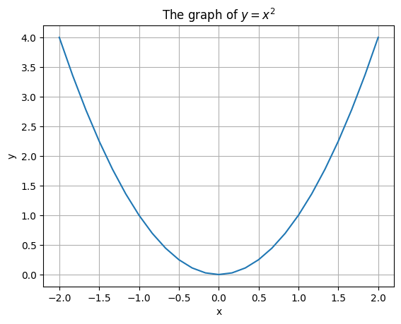
Now let’s graph the function $y = x^2$ over the domain $-2 \leq x \leq 2$ for practice. As a first step, we use numpy’s linspace function to create an evenly spaced set of 11 x-values between -2 and 2.

x_values = numpy.linspace(-2,2,25)  # The argument 11 is the *number* of terms, not the step size!
print(x_values)
type(x_values)

[-2.         -1.83333333 -1.66666667 -1.5        -1.33333333 -1.16666667
 -1.         -0.83333333 -0.66666667 -0.5        -0.33333333 -0.16666667
  0.          0.16666667  0.33333333  0.5         0.66666667  0.83333333
  1.          1.16666667  1.33333333  1.5         1.66666667  1.83333333
  2.        ]

numpy.ndarray

You might notice that the format looks a bit different from a list. Indeed, if you check type(x_values), it’s not a list but something else called a numpy array. Numpy is a package that excels with computations on large arrays of data. On the surface, it’s not so different from a list. The numpy.linspace command is a convenient way of producing an evenly spaced list of inputs.

The big difference is that operations on numpy arrays are interpreted differently than operations on ordinary Python lists. Try the two commands for comparison.

[1,2,3] + [1,2,3]

[1, 2, 3, 1, 2, 3]

x_values + x_values

array([-4.        , -3.66666667, -3.33333333, -3.        , -2.66666667,
       -2.33333333, -2.        , -1.66666667, -1.33333333, -1.        ,
       -0.66666667, -0.33333333,  0.        ,  0.33333333,  0.66666667,
        1.        ,  1.33333333,  1.66666667,  2.        ,  2.33333333,
        2.66666667,  3.        ,  3.33333333,  3.66666667,  4.        ])

y_values = x_values * x_values  # How is multiplication interpreted on numpy arrays?
print(y_values)

[4.         3.36111111 2.77777778 2.25       1.77777778 1.36111111
        0.69444444 0.44444444 0.25       0.11111111 0.02777778
        0.02777778 0.11111111 0.25       0.44444444 0.69444444
        1.36111111 1.77777778 2.25       2.77777778 3.36111111
       ]

Now we use matplotlib to create a simple line graph.

%matplotlib inline
plt.plot(x_values, y_values)
plt.title('The graph of $y = x^2$')  # The dollar signs surround the formula, in LaTeX format.
plt.ylabel('y')
plt.xlabel('x')
plt.grid(True)
plt.show()

../_images/a16bb2e6f94d924fc2b6d62902d6ffe2465f3ff44dfecbc4cef4ffc62bc45de0.png

Let’s analyze the graphing code a bit more. See the official pyplot tutorial for more details.

%matplotlib inline
plt.plot(x_values, y_values)
plt.title('The graph of $y = x^2$')  # The dollar signs surround the formula, in LaTeX format.
plt.ylabel('y')
plt.xlabel('x')
plt.grid(True)
plt.show()

The first line contains the magic %matplotlib inline. We have seen a magic word before, in %timeit. Magic words can call another program to assist. So here, the magic %matplotlib inline calls matplotlib for help, and places the resulting figure within the notebook.

The next line plt.plot(x_values, y_values) creates a plot object based on the data of the x-values and y-values. It is an abstract sort of object, behind the scenes, in a format that matplotlib understands. The following lines set the title of the plot, the axis labels, and turns a grid on. The last line plt.show renders the plot as an image in your notebook. There’s an infinite variety of graphs that matplotlib can produce – see the gallery for more! Other graphics packages include bokeh and seaborn, which extends matplotlib.

4.5.2. Analysis of the prime counting function#

Now, to analyze the prime counting function, let’s graph it. To make a graph, we will first need a list of many values of x and many corresponding values of $\pi(x)$. We do this with two commands. The first might take a minute to compute.

x_values = numpy.linspace(0,1000000,1001) # The numpy array [0,1000,2000,3000,...,1000000]
pix_values = numpy.array([primes_upto(x) for x in x_values])  # [FUNCTION(x) for x in LIST] syntax

We created an array of x-values as before. But the creation of an array of y-values (here, called pix_values to stand for $\pi(x)$) probably looks strange. We have done two new things!

We have used a list comprehension [primes_upto(x) for x in x_values] to create a list of y-values.
We have used numpy.array(LIST) syntax to convert a Python list into a numpy array.

First, we explain the list comprehension. Instead of pulling out values of a list according to a condition, with [x for x in LIST if CONDITION], we have created a new list based on performing a function each element of a list. The syntax, used above, is [FUNCTION(x) for x in LIST]. These two methods of list comprehension can be combined, in fact. The most general syntax for list comprehension is [FUNCTION(x) for x in LIST if CONDITION].

Second, a list comprehension can be carried out on a numpy array, but the result is a plain Python list. It will be better to have a numpy array instead for what follows, so we use the numpy.array() function to convert the list into a numpy array.

type(numpy.array([1,2,3]))  # For example.

numpy.ndarray

Now we have two numpy arrays: the array of x-values and the array of y-values. We can make a plot with matplotlib.

len(x_values) == len(pix_values)  # These better be the same, or else matplotlib will be unhappy.

True

%matplotlib inline
plt.plot(x_values, pix_values)
plt.title('The prime counting function')
plt.ylabel('$\pi(x)$')
plt.xlabel('x')
plt.grid(True)
plt.show()

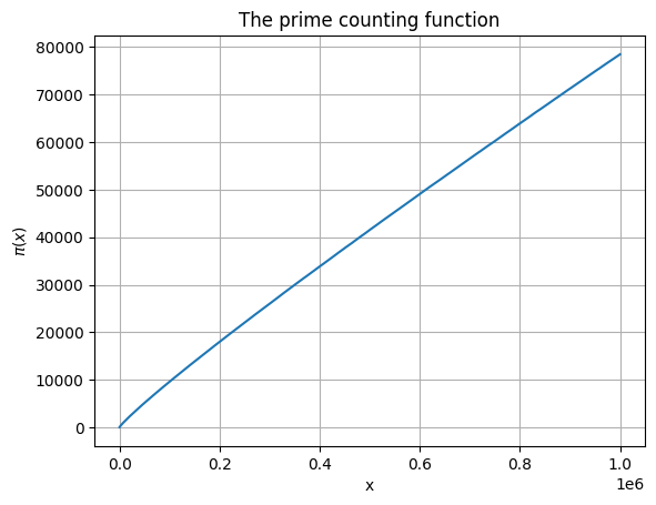
../_images/ea0a7495fad8b199f604e3b613f918ec0c105ff9d05f6de62fb5f7f303a3ff5c.png

In this range, the prime counting function might look nearly linear. But if you look closely, there’s a subtle downward bend. This is more pronounced in smaller ranges. For example, let’s look at the first 10 x-values and y-values only.

%matplotlib inline
plt.plot(x_values[:10], pix_values[:10])  # Look closer to 0.
plt.title('The prime counting function')
plt.ylabel('$\pi(x)$')
plt.xlabel('x')
plt.grid(True)
plt.show()

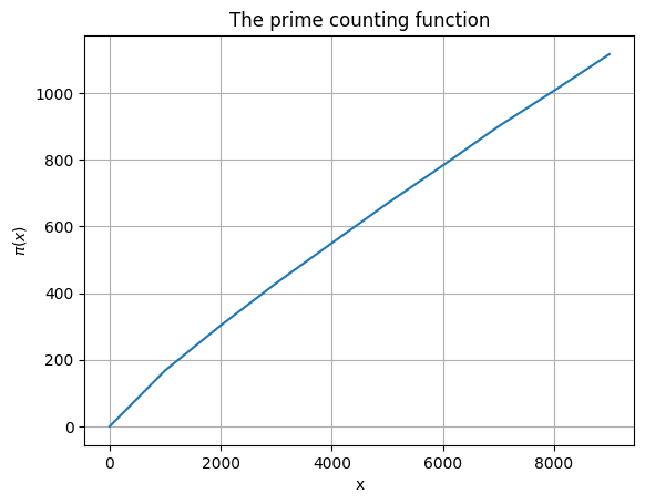
../_images/16553f7fe07fd282000b3629ffba138076a888087e76c7baa471f2cbd5dfdf41.png

It still looks almost linear, but there’s a visible downward bend here. How can we see this bend more clearly? If the graph were linear, its equation would have the form $\pi(x) = mx$ for some fixed slope $m$ (since the graph does pass through the origin). Therefore, the quantity $\pi(x)/x$ would be constant if the graph were linear.

Hence, if we graph $\pi(x) / x$ on the y-axis and $x$ on the x-axis, and the result is nonconstant, then the function $\pi(x)$ is nonlinear.

m_values = pix_values[1:] / x_values[1:]  # We start at 1, to avoid a division by zero error.

%matplotlib inline
plt.plot(x_values[1:], m_values)
plt.title('The ratio $\pi(x) / x$ as $x$ varies.')
plt.xlabel('x')
plt.ylabel('$\pi(x) / x$')
plt.grid(True)
plt.show()

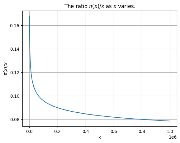
../_images/156b8ef2afe5835718c7a264dfa025ad5af8e26675b8e3517dbfee0d5f08457e.png

That is certainly not constant! The decay of $\pi(x) / x$ is not so different from $1 / \log(x)$, in fact. To see this, let’s overlay the graphs. We use the numpy.log function, which computes the natural logarithm of its input (and allows an entire array as input).

%matplotlib inline
plt.plot(x_values[1:], m_values, label='$\pi(x)/x$')  # The same as the plot above.
plt.plot(x_values[1:], 1 / numpy.log(x_values[1:]), label='$1 / \log(x)$')  # Overlay the graph of 1 / log(x)
plt.title('The ratio of $\pi(x) / x$ as $x$ varies.')
plt.xlabel('x')
plt.ylabel('$\pi(x) / x$')
plt.grid(True)
plt.legend()  # Turn on the legend.
plt.show()

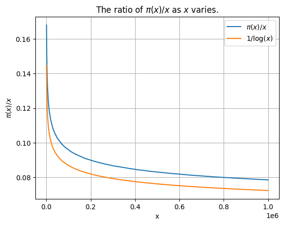
../_images/2536b3dd33b164c4f5310abe3fec57bd2cea8d64784260ce8ef1316c0d6b2f64.png

The shape of the decay of $\pi(x) / x$ is very close to $1 / \log(x)$, but it looks like there is an offset. In fact, there is, and it is pretty close to $1 / \log(x)^2$. And that is close, but again there’s another little offset, this time proportional to $2 / \log(x)^3$. This goes on forever, if one wishes to approximate $\pi(x) / x$ by an “asymptotic expansion” (not a good idea, it turns out).

The closeness of $\pi(x) / x$ to $1 / \log(x)$ is expressed in the prime number theorem: $$\lim_{x \rightarrow \infty} \frac{\pi(x)}{x / \log(x)} = 1.$$

%matplotlib inline
plt.plot(x_values[1:], m_values * numpy.log(x_values[1:])  )  # Should get closer to 1.
plt.title('The ratio $\pi(x) / (x / \log(x))$ approaches 1... slowly')
plt.xlabel('x')
plt.ylabel('$\pi(x) / (x / \log(x)) $')
plt.ylim(0.8,1.2)
plt.grid(True)
plt.show()

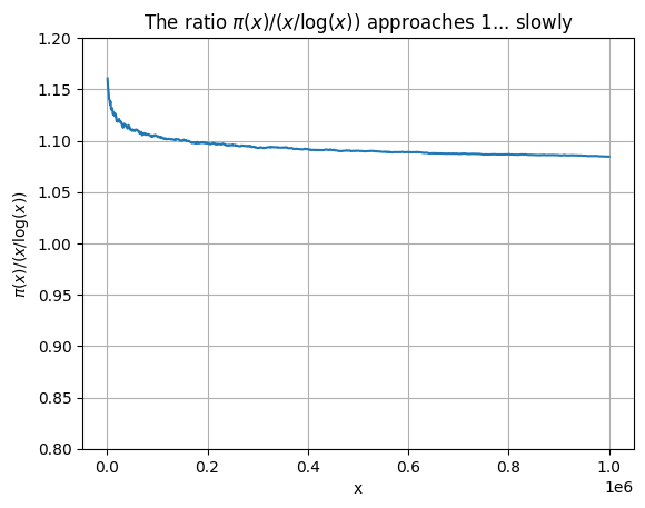
../_images/4ac5aef0443dcd5fc95aa7c079c5c0b691abfdb3fc3f1f52dc8696376cdbaf28.png

Comparing the graph to the theoretical result, we find that the ratio $\pi(x) / (x / \log(x))$ approaches $1$ (the theoretical result) but very slowly (see the graph above!).

A much stronger result relates $\pi(x)$ to the “logarithmic integral” $li(x)$. The Riemann hypothesis is equivalent to the statement $$\left\vert \pi(x) - li(x) \right\vert = O(\sqrt{x} \log(x)).$$ In other words, the error if one approximates $\pi(x)$ by $li(x)$ is bounded by a constant times $\sqrt{x} \log(x)$. The logarithmic integral function isn’t part of Python or numpy, but it is in the mpmath package. If you have this package installed, then you can try the following.

from mpmath import li

print(primes_upto(1000000))  # The number of primes up to 1 million.
print(li(1000000))  # The logarithmic integral of 1 million.

78498
78627.5491594622

4.5.3. Prime gaps#

As a last bit of data analysis, we consider the prime gaps. These are the numbers that occur as differences between consecutive primes. Since all primes except 2 are odd, all prime gaps are even except for the 1-unit gap between 2 and 3. There are many unsolved problems about prime gaps; the most famous might be that a gap of 2 occurs infinitely often (as in the gaps between 3,5 and between 11,13 and between 41,43, etc.).

Once we have our data set of prime numbers, it is not hard to create a data set of prime gaps. Recall that primes is our list of prime numbers up to 1 million.

len(primes) # The number of primes up to 1 million.

primes_allbutlast = primes[:-1]  # This excludes the last prime in the list.
primes_allbutfirst = primes[1:]  # This excludes the first (i.e., with index 0) prime in the list.

primegaps = numpy.array(primes_allbutfirst) - numpy.array(primes_allbutlast) # Numpy is fast!

print(primegaps[:100])  # The first hundred prime gaps!

[ 1  2  2  4  2  4  2  4  6  2  6  4  2  4  6  6  2  6  4  2  6  4  6  8
2  4  2  4 14  4  6  2 10  2  6  6  4  6  6  2 10  2  4  2 12 12  4
4  6  2 10  6  6  6  2  6  4  2 10 14  4  2  4 14  6 10  2  4  6  8
6  4  6  8  4  8 10  2 10  2  6  4  6  8  4  2  4 12  8  4  8  4  6
2 18  6]

What have we done? It is useful to try out this method on a short list.

L = [1,3,7,20]  # A nice short list.

print(L[:-1])
print(L[1:])

[1, 3, 7]
[3, 7, 20]

Now we have two lists of the same length. The gaps in the original list L are the differences between terms of the same index in the two new lists. One might be tempted to just subtract, e.g., with the command L[1:] - L[:-1], but subtraction is not defined for lists. Note that L[1:] - L[:-1] will give a TypeError.

Fortunately, by converting the lists to numpy arrays, we can use numpy’s term-by-term subtraction operation.

numpy.array(L[1:]) - numpy.array(L[:-1])  # See the gaps in the list [1,3,7,20] in the output.

array([ 2,  4, 13])

Now let’s return to our primegaps data set. It contains all the gap-sizes for primes up to 1 million.

print(len(primes))
print(len(primegaps))  # This should be one less than the number of primes.

78498
78497

As a last example of data visualization, we use matplotlib to produce a histogram of the prime gaps.

max(primegaps)  # The largest prime gap that appears!

%matplotlib inline
plt.figure(figsize=(12, 5))  #  Makes the resulting figure 12in by 5in.
plt.hist(primegaps, bins=range(1,115)) #  Makes a histogram with one bin for each possible gap from 1 to 114.
plt.ylabel('Frequency')
plt.xlabel('Gap size')
plt.grid(True)
plt.title('The frequency of prime gaps, for primes up to 1 million')
plt.show()

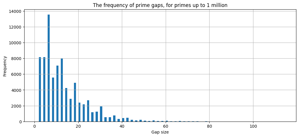
../_images/9c10acee650145b9eca145f0e11ba6e6627393a63a71552abf942aed83429d76.png

Observe that gaps of 2 (twin primes) are pretty frequent. There are over 8000 of them, and about the same number of 4-unit gaps! But gaps of 6 are most frequent in the population, and there are some interesting peaks at 6, 12, 18, 24, 30. What else do you observe?

4.6. Exercises#

To check whether a number n is prime, you can first check whether n is even, and then check whether n has any odd factors. Change the is_prime_fast function by implementing this improvement. How much of a speedup did you get?

def is_prime_fast(n):
    '''
    Checks whether the argument n is a prime number.
    Uses a brute force search for factors between 2 and sqrt(n).
    '''
    j = 2
    root_n = sqrt(n)
    while j <= root_n:  # j will proceed through the list of numbers 2,3,... up to sqrt(n).
        if n%j == 0:  # is n divisible by j?
            print("{} is a factor of {}.".format(j,n))
            return False
        j = j + 1  # There's a Python abbreviation for this:  j += 1.
    return True

Use the %timeit tool to study the speed of is_prime_fast from Exercise 1 for various sizes of n. Using about 10 data points, relate the size of n to the time taken by the is_prime_fast function.
Write a function is_square(n) to test whether a given integer n is a perfect square (like 0, 1, 4, 9, 16, etc.). How fast can you make it run? Describe the different approaches you try and which are fastest.
Create a list L with L = [1,2,3,…,100] (all the numbers from 1 to 100). What is L[50]?
Take the same list L, and extract a slice of the form [5,10,15,…,95] with a command of the form L[a:b:c].
Take the same list L, and change all the even numbers to zeros, so that L looks like [1,0,3,0,5,0,…,99,0]. Hint: You might wish to use the list [0]*50.
Try the command L[-1::-1] on a list. What does it do? Can you guess before executing it? Can you understand why? In fact, strings are indexed like lists. Try setting L = 'Hello' and the previous command.
Create the list [1,100,3,98,5,96,…,99,2], where the odd terms are in order and the even terms are in reverse order. There are multiple methods!
Use the append method with a loop to create a list of perfect squares, [0,1,4,9,16,25,…,10000].
Create a list of 52 “cards” to resemble a standard card deck. The suits can be denoted C,S,D,H for clubs, spades, diamonds, and hearts. The numbers can be denoted 1-13 (with Ace = 1, Jack = 11, Queen = 12, King = 13). So “9H” would be the 9 of hearts, and 12S the queen of spades. Your list L should contain every card.
Challenge: write a function which performs a “perfect riffle shuffle” on a list of cards. This shuffle should have the effect of dividing the deck into two equal pieces, and then precisely interlacing the two pieces to form a new list. E.g., an input list of [1,2,3,4,5,6] should be broken into [1,2,3] and [4,5,6] and then interlaced as [1,4,2,5,3,6].
Prove that the length of range(p*p, n, 2*p) equals $\lfloor \frac{n - p^2 - 1}{2p} \rfloor + 1$.
A natural number $n$ is called squarefree if it has no perfect square divides $n$ except for 1. Write a function squarefree_list(n) which outputs a list of booleans: True if the index is squarefree and False if the index is not squarefree. For example, if you execute squarefree_list(12), the output should be [False, True, True, True, False, True, True, True, False, False, True, True, False]. Note that the False entries are located the indices 0, 4, 8, 9, 12. These natural numbers have perfect square divisors besides 1.
Your DNA contains about 3 billion base pairs. Each “base pair” can be thought of as a letter, A, T, G, or C. How many bits would be required to store a single base pair? In other words, how might you convert a sequence of booleans into a letter A,T,G, or C? Given this, how many megabytes or gigabytes are required to store your DNA? How many people’s DNA would fit on a thumb-drive?
Create functions redprimes_upto(x) and blueprimes_upto(x) which count the number of red/blue primes up to a given number x. Recall that we defined red/blue primes to be those of the form 4n+1 or 4n+3, respectively. Graph the relative proportion of red/blue primes as x varies from 1 to 1 million. E.g., are the proportions 50%/50% or 70%/30%, and how do these proportions change? Note: this is also visualized in An Illustrated Theory of Numbers and you can read an article by Rubinstein and Sarnak for more.
Does there seem to be a bias in the last digits of primes? Note that, except for 2 and 5, every prime ends in 1,3,7, or 9. Note: the last digit of a number n is obtained from n % 10.
Read about the “Prime Conspiracy”, recently discovered by Lemke Oliver and Soundararajan. Can you detect their conspiracy in our data set of primes?